Automatic Differentiation

Posted on September 30, 2010 by azumih

A couple of months ago, I wrote a piece of programme that computes integrals of

polynomials,
products of polynomials, and
compositions of polynomials.

It helped me a bit in that I did not need to expand complicated expressions by hand. The programme could handle my problem somewhat automatically. But the programme was not very interesting in itself…

Lately I saw a nice thing that goes in the opposite direction, differentiation. It is an article in SIAM Review about “automatic differentiation“, which can be downloaded publicly from this site. Its accompanying code written in Matlab is also freely available.

It seems like there are already a lot of software libraries for automatic differentiation in other languages. But they are somewhat big and a bit tough to see what is going on inside them.

So here is a small trial implementation, just for my fun:

#include <cmath>

struct Var
{
 Var(double v = 0) : v(v) {}
 virtual ~Var() {}
 double operator()() const { return v; }
protected:
 double v;
};

struct Fun : Var
{
 Fun() {}
 Fun(Var const& v) : Var(v), d(1) {}
 Fun(double v, double d) : Var(v), d(d) {}
 double D() const { return d; }
protected:
 double d;
};

inline Fun operator*(double c, Var const& v)
{   return Fun(c*v(), c);   }

inline Fun pow(Var const& v, double e)
{   return Fun(std::pow(v(), e), e*std::pow(v(), e - 1)); }

inline Fun operator+(Fun const& f, double c)
{   return Fun(f() + c, f.D()); }

inline Fun operator*(double c, Fun const& f)
{   return Fun(c*f(), c*f.D()); }

inline Fun operator-(Fun const& f)
{   return Fun(-f(), -f.D()); }

inline Fun operator+(Fun const& a, Fun const& b)
{   return Fun(a() + b(), a.D() + b.D()); }

inline Fun operator*(Fun const& a, Fun const& b)
{   return Fun(a() * b(), a.D()*b() + a()*b.D()); }

inline Fun operator/(Fun const& a, Fun const& b)
{   return Fun(a() / b(), (a.D()*b() - a()*b.D())/(b()*b())); }

inline Fun exp(Fun const& f)
{   return Fun(std::exp(f()), std::exp(f())*f.D()); }

inline Fun sin(Fun const& f)
{   return Fun(std::sin(f()), std::cos(f())*f.D()); }

inline Fun cos(Fun const& f)
{   return Fun(std::cos(f()), -std::sin(f())*f.D()); }

// ... and more elementary functions will follow ...

Let me see if this works:

#include <iostream>
#include <iomanip>
int main()
{
 Var x(3.141592653589793);

 Fun f = pow(x, 2) + 2*x + 3;
 std::cout << "val: " << f() << ", der: " << f.D() << std::endl;

 Fun g = 2*exp(sin(x)) + x;
 std::cout << "val: " << g() << ", der: " << g.D() << std::endl;

 Fun h = x/x;
 std::cout << "val: " << h() << ", der: " << h.D() << std::endl;
}

The test above produced these outputs:

val: 19.1528, der: 8.28319
val: 5.14159, der: -1
val: 1, der: 0

This programme seems like working thus far.

Afterthoughts

The class “Var” may not be necessary. But I could not come up with nice small implementation without it.
It may be considered bad to derive “Fun” from “Var”.
Initially, I thought I should start writing this in Python. But it turned out that it is easier to write in C++, thanks to its function overloading feature.
It is awkward that I got to assign a value of independent variable before defining functions whose derivatives are to be evaluated.

lll

Fourier… 2

Posted on September 30, 2010 by azumih

Let me resume the Fourier thing.

Back and forth transform pair are:

$\displaystyle f(x) = \dfrac{1}{2\pi} \int_{-\infty}^{\infty} \hat{f}(\omega) e^{i\omega x} d\omega$ ,

$\displaystyle \hat{f}(\omega) = \int_{-\infty}^{\infty} f(x) e^{-i\omega x} dx$ .

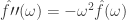
Since I was concerning about solving ODE using Fourier transform in a similar manner as Lapalce’s, I want to see what the Fourier transform of derivatives (with respect to $x$ ) of $f(x)$ look like. For the 1st derivative, I get:

$\displaystyle\hat{f\prime}(\omega) = \int_{-\infty}^{\infty} f\prime(x) e^{-i\omega x} dx = [f(x) e^{-i\omega x}]_{-\infty}^{\infty} -\int_{-\infty}^{\infty} f(x) (e^{-i\omega x})\prime dx$ .

by using integration by parts. If $f(x)$ vanishes at infinity ( $\lim_{x \to \pm \infty}f(x) = 0$ ), then the 1st term becomes 0, so I get:

$\displaystyle\hat{f\prime}(\omega) = -\int_{-\infty}^{\infty} f(x) (e^{-i\omega x})\prime dx = i\omega \int_{-\infty}^{\infty} f(x) e^{-i\omega x} dx = i\omega \hat{f}(\omega)$

Now higher derivatives are easy. Fourier transform of the 2nd derivative, for example, is:

$\displaystyle \hat{f\prime\prime}(\omega) = -\omega^2 \hat{f}(\omega)$ .

Okay. Let me pick a 2nd order ODE:

$\displaystyle u\prime\prime(x) + au\prime(x) + bu(x) = v(x)$ .

Taking Fourier transform of both sides, I get:

$\displaystyle -\omega^2 \hat{u} + i a \omega \hat{u} + b\hat{u} = \hat{v}$ ,

$\displaystyle \hat{u}(\omega) = \dfrac{\hat{v}(\omega)}{-\omega^2 + i a \omega + b}$ .

Finally I reach $f(x)$ by inverse-transforming both sides:

$\displaystyle u(x) = \dfrac{1}{2\pi}\int_{-\infty}^{\infty} \dfrac{\hat{v}(\omega)}{-\omega^2 + i a \omega + b} e^{i\omega x} d\omega$ .

mmm… but is the integral on the right hand side looks so clumsy… It is a double-integral actually.

Fourier, Laplace…

Posted on September 25, 2010 by azumih

Again this is quasi-mathematical imprecise thoughts about blah blah transforms.

I saw a book that has both Fourier and Laplace transforms in its title. The book says that Laplace transform is a generalisation of Fourier transform, in something like this way…

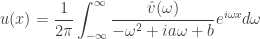Let’s say $x(t)$ is a function that has such and such nice properties. Then there is another function $X(\omega)$ such that

$\displaystyle X(\omega) = \int_{-\infty}^\infty x(t) e^{-i \omega t}dt$ ,

which is called Fourier transform of $x(t)$ .

Then letting $i \omega = s$ , we have

$\displaystyle X(s) = \int_{-\infty}^\infty x(t) e^{-st}dt$ ,

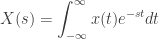which is called Lapalce trasnform. —I think $X(\omega)$ should have been $X(-i \omega)$ to make the things more straight.

Okay. The point is taken. $s$ is simpler than $i\omega$ . I must admit Laplace transform is more general. This seemed to be all spoken about relation between Fourier and Laplace transforms in the book.

But wait a second. Usually Laplace transform is introduced to us as a means for solving initial value problems of differential equations, isn’t it? I thought Fourier transform also should be talked about as a similar method for solving IVPs, to make relationship between these trasnforms clearer…

Radon and Hough Transform

Posted on September 8, 2010 by azumih

Image via Wikipedia

This is to follow-up my earlier post.

In computed tomography of 2D parallel projection, its scanning process can be regarded as a real world example of 2D Radon transform. Let us call density function (or beam attenuation coefficient or beam absorption coefficient) of body to be scanned $f(x, y)$ . Then scanned data for each projection angle $\theta$ , after correcting exponential decay of beam due to attenuation, can be seen as Radon transform of $f(x, y)$ :

$\displaystyle Rf(\theta, X) = \int_{-\infty}^\infty f(X \cos \theta -Y \sin \theta, X \sin \theta + Y \cos \theta) dY.$

Where $(X, Y)$ are rotated coordinates:

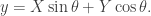
$\displaystyle x = X \cos \theta -Y \sin \theta,$
$\displaystyle y = X \sin \theta + Y \cos \theta.$

Taking Fourier transform of $f(x, y)$ we get:

$\displaystyle F(\xi, \eta) = \int_{-\infty}^\infty \int_{-\infty}^\infty f(x, y) e^{-i(\xi x + \eta y)} dx dy.$

Then $F(\xi, \eta)$ in polar coordinates $\xi = w \cos \theta, \eta = w \sin \theta$ would look like:

$\displaystyle F(w \cos \theta, w \sin \theta) = \int_{-\infty}^\infty \int_{-\infty}^\infty f(x, y) e^{-i(\xi x + \eta y)} dx dy.$

I want to change variables from $(x, y)$ to $(X, Y)$ in order to relate $F$ to the Radon transform $Rf$ . Because of the change to polar coordinates, the exponent $\xi x + \eta y$ becomes:

$\displaystyle \xi x + \eta y = xw\cos \theta + yw \sin \theta = w(x \cos \theta + y \sin \theta) = wX$ .

And Jacobian is:

$\displaystyle \dfrac{\partial x \partial y}{\partial X \partial Y} = \left | \begin{array}{ccc} \cos \theta & -\sin \theta \\ \sin \theta & \cos \theta \end{array} \right | = 1$ .

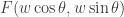So $F(w \cos \theta, w \sin \theta)$ is rewritten as:

$\displaystyle F(w \cos \theta, w \sin \theta) = \int_{-\infty}^\infty [ \int_{-\infty}^\infty f(X \cos \theta - Y \sin \theta, X \sin \theta + Y \cos \theta) dY ] e^{-iwX} dX$ .

Gazing the inner integral with respect to Y for a while… carefully… This is just the projection of $f$ in the direction of $\theta$ , which is… Radon transform:

$\displaystyle F(w \cos \theta, w \sin \theta) = \int_{-\infty}^\infty Rf(\theta, X) e^{-iwX} dX$ .

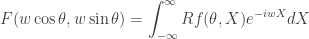Okay, finally gazing this last integral for another while… patiently… It turns out that this is rightly Fourier transform of $Rf$ with respect to $X$ , doesn’t it? My boss used to call this “Fourier slice theorem” or “central slice theorem“. In CT, “filtered back projection” is a most important method for reconstructing $f(x, y)$ from projection data $Rf(\theta, X)$ , and the method is based on the slice theorem.

But this theorem does not force us to go only backward (reconstruction) . If we have an image $f(x, y)$ at hand, then we can go forward to get lots of projection data using the same theorem. Getting lots of projection data is same thing as plotting on $(r, \theta)$ plane in Hough transform. Steps to get projections using this idea are:

Fourier transform the $f(x, y)$ –> $F$ ,
Resample $F$ radially to convert to polar coordinates –> $P$ ,
Inverse Fourier transform $P$ –> projection data $p$ .

Proper resampling should be difficult in practice. It is like filtering in filtered back projection is difficult. But I think it is still nice to be aware of the theorem, maybe just for fun.

weblogger.el

Posted on September 2, 2010 by azumih

trying to post from within emacs…

0909

und sofort ins unendliche

Monthly Archives: September 2010