

Image via Wikipedia
This is to follow-up my earlier post.
In computed tomography of 2D parallel projection, its scanning process can be regarded as a real world example of 2D Radon transform. Let us call density function (or beam attenuation coefficient or beam absorption coefficient) of body to be scanned 


Where 

Taking Fourier transform of 

Then 


I want to change variables from 


And Jacobian is:

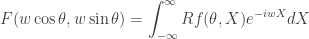
So 
![\displaystyle F(w \cos \theta, w \sin \theta) = \int_{-\infty}^\infty [ \int_{-\infty}^\infty f(X \cos \theta - Y \sin \theta, X \sin \theta + Y \cos \theta) dY ] e^{-iwX} dX](https://s0.wp.com/latex.php?latex=%5Cdisplaystyle+F%28w+%5Ccos+%5Ctheta%2C+w+%5Csin+%5Ctheta%29+%3D+%5Cint_%7B-%5Cinfty%7D%5E%5Cinfty+%5B+%5Cint_%7B-%5Cinfty%7D%5E%5Cinfty+f%28X+%5Ccos+%5Ctheta+-+Y+%5Csin+%5Ctheta%2C+X+%5Csin+%5Ctheta+%2B+Y+%5Ccos+%5Ctheta%29+dY+%5D+e%5E%7B-iwX%7D+dX&bg=ffffff&fg=333333&s=0&c=20201002)
Gazing the inner integral with respect to Y for a while… carefully… This is just the projection of 
Okay, finally gazing this last integral for another while… patiently… It turns out that this is rightly Fourier transform of 

But this theorem does not force us to go only backward (reconstruction) . If we have an image 
- Fourier transform the
- Resample
,
- Inverse Fourier transform
.
Proper resampling should be difficult in practice. It is like filtering in filtered back projection is difficult. But I think it is still nice to be aware of the theorem, maybe just for fun.
